Class Activation Map
This demo shows the method proposed in Learning Deep Features for Discriminative Localization
This is an R port of the Python demo found here.
Idea is to apply the last fully connected layer to each of the pixel following the last convolution layer. In Resnet, this applies to the 7x7 final features, just before the global average pooling.
Since the final FC is meant to create a score for each of the 1000 classes, applying those FC weights to the 7x7features prior their pooling result in a class score for each of those pixel.
require("grid")
require("readr")
require("dplyr")
require("plotly")
require("imager")
require("mxnet")
Load model
A ResNet model is loaded and its last convolution output is grouped together the softmax output. Also, the weights of the last fully connected output is extracted.
These are the key ingredients of the class activation map.
resnet <- mx.model.load("../models/resnet-50", iteration=0)

labels_resnet <- readLines("../models/synset.txt")
labels_resnet <- gsub(pattern = "(n\\d+\\s)(.+)", replacement="\\2", x=labels_resnet)

symbol <- resnet$symbol
internals <- symbol$get.internals()
outputs <- internals$outputs

# last layer before global pooling
conv <- internals$get.output(which(outputs=="relu1_output"))
# flatten layer
softmax <- internals$get.output(which(outputs=="softmax_output"))
symbol_group <- mx.symbol.Group(c(conv, softmax))
# last fully connected weights
weight_fc <- resnet$arg.params$fc1_weight
Image treatment
Add padding to image and reshape into a 224 X 224 as required by ResNet model.
preproc_resnet_pad <- function(im, resize=224) {
  shape <- dim(im)[1:2]
  axis = c("x", "y")[which.min(shape)]
  pad = abs(diff(shape))
  im <- pad(im, nPix=pad, axes = axis)
  resized <- resize(im, resize, resize)
  array <- as.array(resized) * 255
  dim(array) <- c(resize, resize, 3, 1)
  return(array)
}

im <- imager::load.image("../models/cat-dog-2.jpg")

data_array <- preproc_resnet_pad(im)
data = mx.nd.array(data_array)
label = mx.nd.array(1)

im_array <- data_array
dim(im_array) <- dim(im_array)[1:3]
plot(im_array %>% as.cimg())
## Warning in as.cimg.array(.): Assuming third dimension corresponds to colour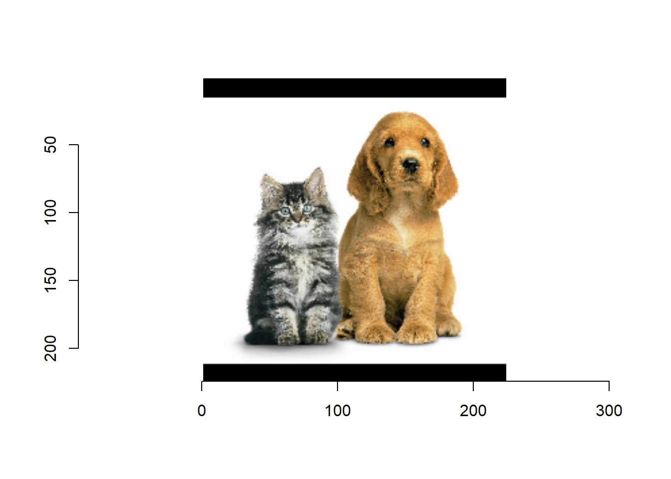
Generate activation map
arg_names <- symbol_group$arguments
arg.arrays <- c(list(data=data, softmax_label = label), resnet$arg.params)[arg_names]
aux.arrays <- resnet$aux.params[symbol_group$auxiliary.states]

# outputs = mod.predict(blob)
exec <- mxnet:::mx.symbol.bind(symbol = symbol_group, ctx = mx.cpu(),
                                 arg.arrays = arg.arrays,
                                 aux.arrays = aux.arrays,
                                 grad.reqs = rep("null", length(arg.arrays)))

mx.exec.forward(exec, is.train = F)
outputs <- exec$outputs
score = outputs[[2]]
conv_fm = outputs[[1]]
dim(conv_fm)
## [1] 7 7 2048 1# get the indices of the topk predictions
top_k = 8
inds_topk <- mx.nd.topk(data=score, axis=1, k=top_k) %>% mx.nd.reshape(-1)
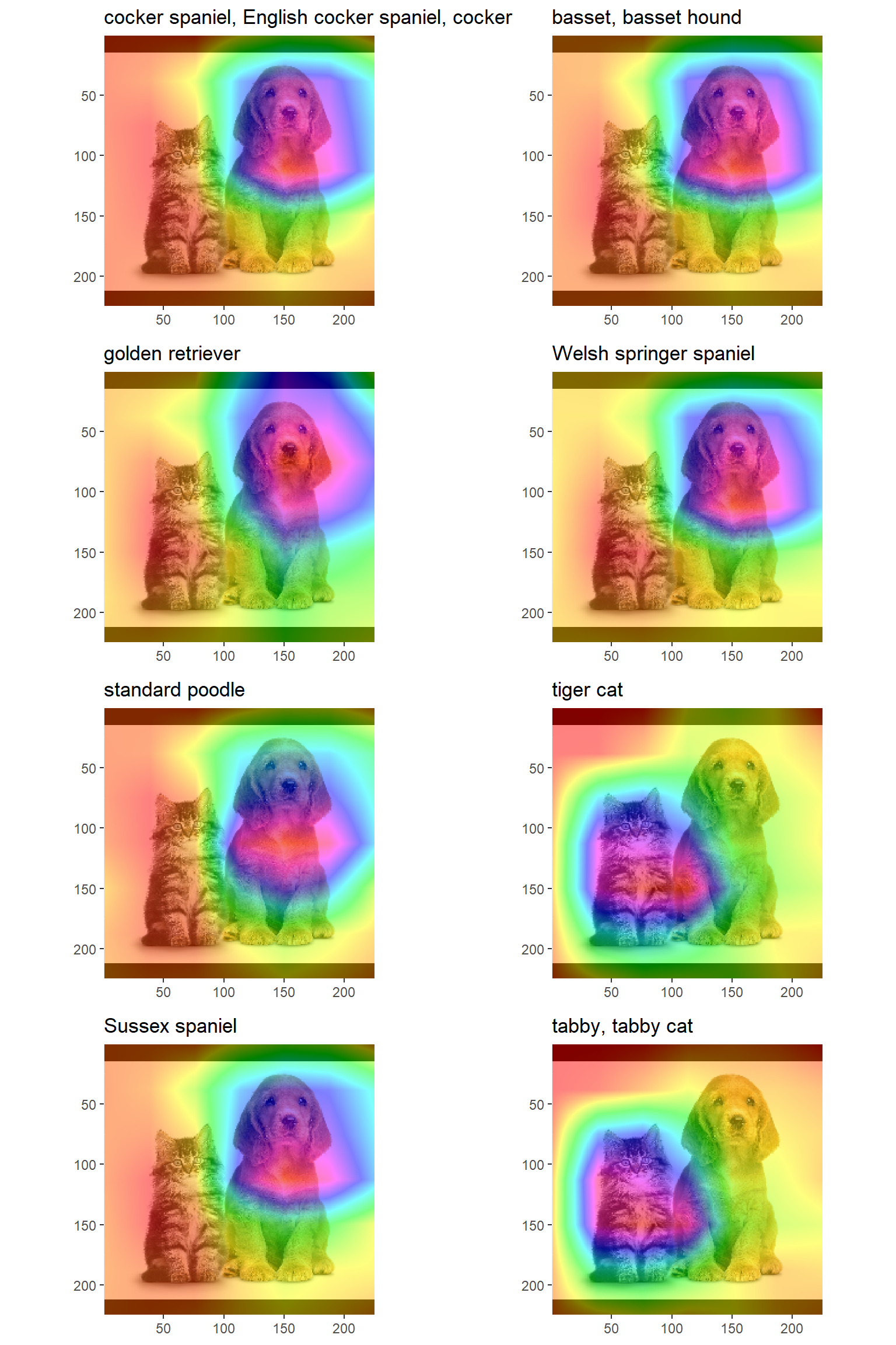
labels_resnet[as.array(inds_topk)+1]## [1] "cocker spaniel, English cocker spaniel, cocker"
## [2] "golden retriever"
## [3] "standard poodle"
## [4] "Sussex spaniel"
## [5] "basset, basset hound"
## [6] "Welsh springer spaniel"
## [7] "tiger cat"
## [8] "tabby, tabby cat"CAM function
Apply the last fully connected operation to each of the final 7x7 features. Only the weights relevant to the top k classes are kept from the FC weights.
get_cam <- function(conv_fm, weight_fc) {

  conv_fm = mx.nd.reshape(data = conv_fm, shape = c(0,0,0), reverse = T)
  conv_fm_flatten = mx.nd.reshape(data = conv_fm, shape = c(-1,0))
  dim(conv_fm)
  dim(conv_fm_flatten)
  dim(weight_fc)

  # results in shape (height X width) X topk
  detection_map = mx.nd.dot(lhs = weight_fc, rhs = conv_fm_flatten)
  map_shapes <- dim(detection_map)
  detection_map = mx.nd.reshape(detection_map, shape=c(sqrt(map_shapes[1]), sqrt(map_shapes[1]), map_shapes[2]))
  return(detection_map)
}
Plot activation map
Plot image with activation mask for the top 4 labels.
weight_fc_topk = mx.nd.take(weight_fc, indices = inds_topk, axis = 0)
cam = get_cam(conv_fm = conv_fm, weight_fc = weight_fc_topk)
cam_array = cam %>% as.array()
ori_image = im_array %>% as.cimg()
## Warning in as.cimg.array(.): Assuming third dimension corresponds to colourori_image = ori_image / max(ori_image)
plots <- list()
for (k in 1:top_k) {
cam_img = cam_array[, , k] %>% as.cimg()
heat_map = resize(cam_img, size_x = dim(im_array)[1], size_y = dim(im_array)[1], interpolation_type = 3)
max_response = mean(cam_img)
heat_map_color = hsv(h = (heat_map - min(heat_map))/(max(heat_map) - min(heat_map))) %>%
col2rgb %>% t %>% as.vector %>% as.cimg(dim=c(dim(heat_map)[1:3],3))
heat_map_color <- heat_map_color / 255
im_comb <- imdraw(ori_image, heat_map_color, opacity = 0.5)
df <- as.data.frame(im_comb,wide="c") %>% mutate(rgb.val=rgb(c.1,c.2,c.3))
p <- ggplot(df,aes(x,y))+geom_raster(aes(fill=rgb.val))+scale_fill_identity()
p <- p+scale_x_continuous(expand=c(0,0))+scale_y_continuous(expand=c(0,0),trans=scales::reverse_trans()) + ggtitle(labels_resnet[as.array(inds_topk)+1][k])+coord_fixed(ratio = 1) +
theme(axis.title=element_blank())
plots[[k]] <- p
}
multiplot(plotlist = plots, cols = 2)